Impact Factor ISSN: 1449-1907

 Global reach, higher impact
Int J Med Sci 2013; 10(11):1459-1461. doi:10.7150/ijms.6455 This issue Cite
Short Research Communication
Evaluating Epidemiological Evidence: A Simple Test
Wenbin Liang ![]()
National Drug Research Institute, Curtin University, Perth, Western Australia, Australia
Received 2013-4-12; Accepted 2013-8-12; Published 2013-8-28
Abstract
Epidemiological studies that investigate the relationships between health behaviors and diseases may be affected by both known and unknown confounding factors. Alcohol use is one of these behaviors that have been intensively investigated in epidemiological studies. This manuscript introduced a simple test that can identify confounded epidemiological studies. This approach is sensitive to both known and unknown confounders. It provides a new perspective to develop measures for evidence selection in the future.
Keywords: evidence-based medicine, bias, epidemiology, causality, health behaviors
Some human behaviors are at least partly influenced by individuals' own health [1, 2]. For example people tend to quit or reduce their alcohol use when they experience ill health [3-5]. For cohort studies that investigate alcohol use and chronic disease outcomes, the influence of health on drinking behaviors could produce strong confounding effects which are difficult to block through multivariate analysis. It is impossible to tell whether the adjusted results are still manipulated by confounders or not. The following paragraphs will introduce a user-friendly test that tags confounded estimations.
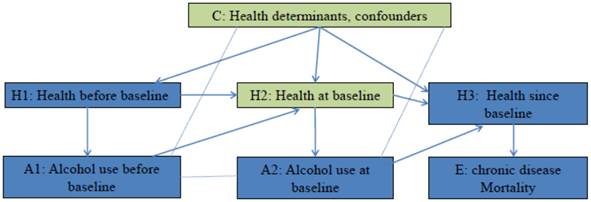
The hypothesis that alcohol use at baseline affects mortality of chronic disease has been studied in many cohort studies [6]. Figure 1 employed the concept of casual diagrams developed by Pearl and Colleagues [7, 8] to illustrate the connections. It is hypothesized that Alcohol use at baseline (A2) affects mortality of chronic disease (E) through its biological effects on health after baseline (H3), and alcohol use before baseline (A1) affects mortality of chronic disease (E) through its biological effects on health at baseline (H2), which further affects health after baseline (H3). On the other hand, health influences people's drinking behaviors. In Figure 1, Health before baseline (H1) affects alcohol use before baseline (A1), and health at baseline (H2) affects alcohol use at baseline (A2). To investigate the effect of A2 on E, the confounding effects of H2 and other confounders (C) have to be blocked. If this hypothesis is tested in a randomized control trial, participants are randomly assigned to groups with different level of alcohol use since baseline. Randomization blocks confounding effects of health status and other factors, therefore any difference in mortality between groups is a result of difference in alcohol use. In cohort studies, alcohol use levels are self-determined. Multivariate analysis is conducted to block confounding effects of H2 and C. If effect of H2 and C is successfully blocked, the effect of A1 and H1 that passes through H2 will be blocked as well. This means for a given alcohol use level at baseline, the estimated risk will not be differed/affected by alcohol use before baseline (A1). In other words, the adjusted risk among participants with the same alcohol use level at baseline is expected to be the same regardless their alcohol use prior to baseline, if all confounding effects are removed. The mirror scenario in randomized controlled trial is that when testing the effects of a drug on a secondary event, possible confounding effect of prior medication use has to be removed (through randomization) [9]. Therefore within the same level of baseline alcohol use, any variation in adjusted risk estimates by prior alcohol use indicates the present of confounding effects. For example, most studies that compared the risk of chronic disease mortality between lifelong abstainers and former drinkers, observed risk difference between the two groups [6], and therefore the estimations from these studies are biased.
Testing the hypothesis: does alcohol use at baseline affect the mortality of chronic disease? Arrow line: Causal association, the direction of arrow indicates the cause-to-outcome direction. Dot line without arrow: Correlation
Data in Table 1 and Estimations in Table 2 provide a simple example to illustrate the general application of this confounding effect detection test. Let's assume that i) this study is to investigate the effect of a dietary supplement on the mortality; ii) the dietary supplement increases the mortality by 100%, so that the exposed-to-unexposed risk ratio equals to 2; iii) there were only three different risk levels at baseline: I1= 1 per 100 person years, I2=3 per 100 person years and I3= 5 per 100 person years. When randomization is applied, it is not necessary to control or stratify for the confounding effects, and the non-stratified exposed-to-unexposed risk ratio provides an unbiased estimate (Estimation 1).
Data for demonstration
| Risk level at baseline | Exposure before baseline | Exposure at baseline | |||
|---|---|---|---|---|---|
| non-user | user | ||||
| person-years | cases | Person-years | cases | ||
| Randomization in place (corresponding to Estimation 1) | |||||
| I1 | non-user | 10000 | 100 | 10000 | 200 |
| user | 15000 | 150 | 15000 | 300 | |
| Subtotal | 25000 | 250 | 25000 | 500 | |
| I2 | non-user | 7500 | 225 | 7500 | 450 |
| user | 7500 | 225 | 7500 | 450 | |
| Subtotal | 15000 | 450 | 15000 | 900 | |
| I3 | non-user | 2500 | 125 | 2500 | 250 |
| user | 7500 | 375 | 7500 | 750 | |
| Subtotal | 10000 | 500 | 10000 | 1000 | |
| Non-randomized, Correct stratification of confounding effects (corresponding to Estimation 2, 3) | |||||
| I1 | non-user | 6000 | 60 | 14000 | 280 |
| user | 6000 | 60 | 24000 | 480 | |
| Subtotal | 12000 | 120 | 38000 | 760 | |
| I2 | non-user | 7500 | 225 | 7500 | 450 |
| user | 7500 | 225 | 7500 | 450 | |
| Subtotal | 15000 | 450 | 15000 | 900 | |
| I3 | non-user | 4000 | 200 | 1000 | 100 |
| user | 12000 | 600 | 3000 | 300 | |
| Subtotal | 16000 | 800 | 4000 | 400 | |
| Non-randomized, Incorrect stratification of confounding effects (corresponding to Estimation 4) | |||||
| I1 | non-user | 6000 | 60 | 14000 | 280 |
| user | 6000 | 60 | 24000 | 480 | |
| Subtotal | 12000 | 120 | 38000 | 760 | |
| I2 and I3 | non-user | 11500 | 425 | 8500 | 550 |
| user | 19500 | 825 | 10500 | 750 | |
| Subtotal | 31000 | 1250 | 19000 | 1300 | |
Estimations of risk ratios based on data in table 1
| Estimation 1 | [(500+900+1000)/(25000+15000+10000)]/[(250+450+500)/(25000+15000+10000)]=2 |
| Estimation 2 | [(760+900+400)/(38000+15000+4000)]/[(120+450+800)/(12000+15000+16000)]=1.13 |
| Test 1 | [(60+225+600)/(6000+7500+12000)]/[(60+225+200)/(6000+7500+4000)]=1.25 |
| Estimation 3 | (760/38000)/(120/12000)=2; (900/15000)/(450/15000)=2; (400/4000)/(800/16000)=2; Weighted estimate = 2 |
| Test 2 | (60/6000)/(60/6000)=1; (225/7500)/(225/7500)=1; (600/12000)/(200/4000)=1. |
| Estimation 4 | (760/38000)/(120/12000)=2; (1300/19000)/(1250/31000)=1.69; Weighted estimate= 1.74. |
| Test 3 | (60/6000)/(60/6000)=1; (825/19500)/(425/11500)=1.14. |
If randomization is not available, non-stratified exposed-to-unexposed risk ratio produces a biased estimate (Estimation 2), and the presence of confounding effects will be detected by the test: the risk ratio by previous exposure status among non-users at baseline does not equal to 1 (= 1.25) (Test 1).
If the stratification of confounding effects is performed precisely, the confounding effects will be fully blocked (Estimation 3). In this case the risk ratio by previous exposure status among non-users at baseline equals to 1, which indicates the absence of residual confounding effects (Test 2).
If the stratification for confounding effect is not performed correctly, there will be residual confounding effects (Estimation 4). The presence of confounding effects will be detected by the test: the risk ratio by previous exposure among non-users at baseline does not equal to 1 (= 1.14) (Test 3).
Furthermore, it is rarely possible to assume that all confounding factors are known or measured in a given observational study. However this test can detect the effects of confounding factors without identifying these factors, and therefore it is effective towards unknown confounding factors.
Competing Interests
The author has declared that no competing interest exists.
References
1. Lemon SC, Zapka JG, Clemow L. Health behavior change among women with recent familial diagnosis of breast cancer. Preventive Medicine. 2004;39:253-62 doi:10.1016/j.ypmed.2004.03.039
2. Baranowski T, Cullen KW, Nicklas T, Thompson D, Baranowski J. Are Current Health Behavioral Change Models Helpful in Guiding Prevention of Weight Gain Efforts? Obesity Research. 2003;11:23S-43S doi:10.1038/oby.2003.222
3. Rehm J, Irving H, Ye Y, Kerr WC, Bond J, Greenfield TK. Are lifetime abstainers the best control group in alcohol epidemiology? On the stability and validity of reported lifetime abstention. Am J Epidemiol. 2008;168:866-71 doi:10.1093/aje/kwn093
4. Shaper AG, Wannamethee G, Walker M. Alcohol and mortality in British men: explaining the u-shaped curve. The Lancet. 1988;332:1267-73
5. Liang W, Chikritzhs T. Reduction in alcohol consumption and health status. Addiction. 2011;106:75-81 doi:10.1111/j.1360-0443.2010.03164.x
6. Fillmore KM, Kerr WC, Stockwell T, Chikritzhs T, Bostrom A. Moderate alcohol use and reduced mortality risk: Systematic error in prospective studies. Addiction Research and Theory. 2006;14:101-32
7. Greenland S, Pearl J, Robins JM. Causal Diagrams for Epidemiologic Research. Epidemiology. 1999;10:37-48 doi:10.2307/3702180
8. PEARL J. Causal diagrams for empirical research. Biometrika. 1995;82:669-88 doi:10.1093/biomet/82.4.669
9. The ESPRIT Study Group. Aspirin plus dipyridamole versus aspirin alone after cerebral ischaemia of arterial origin (ESPRIT): randomised controlled trial. The Lancet. 2006;367:1665-73 doi:10.1016/S0140-6736(06)68734-5
Author contact
![]() Corresponding author: Wenbin Liang, National Drug Research Institute, Curtin University, GPO Box U1987, Perth WA 6845 Australia. Phone: +61 8 9266 1617; Fax: +61 8 9266 1611; Email: w.liangedu.au
Corresponding author: Wenbin Liang, National Drug Research Institute, Curtin University, GPO Box U1987, Perth WA 6845 Australia. Phone: +61 8 9266 1617; Fax: +61 8 9266 1611; Email: w.liangedu.au