PDF

Int J Med Sci 2004; 1(2):63-75. doi:10.7150/ijms.1.63 This issue Cite

Monte Carlo Commissioning of Low Energy Electron Radiotherapy Beams using NXEGS Software

Joseph A. Both , Todd Pawlicki

Department of Radiation Oncology, Stanford University School of Medicine, Stanford, CA 94305, USA

Abstract

This work is a report on the commissioning of low energy electron beams of a medical linear accelerator for Monte Carlo dose calculation using NXEGS software (NXEGS version 1.0.10.0, NX Medical Software, LLC). A unique feature of NXEGS is automated commissioning, a process whereby a combination of analytic and Monte Carlo methods generates beam models from dosimetric data collected in a water phantom. This study uses NXEGS to commission 6, 9, and 12 MeV electron beams of a Varian Clinac 2100C using three applicators with standard inserts. Central axis depth-dose, primary axis and diagonal beam profiles, and output factors are the measurements necessary for commissioning of the code. We present a comparison of measured dose distributions with the distributions generated by NXEGS, using confidence limits on seven measures of error. We find that confidence limits are typically less than 3% or 3 mm, but increase with increasing source to surface distance (SSD) and depth at or beyond R₅₀. We also investigate the dependence of NXEGS' performance on the size and composition of data used to commission the program, finding a weak dependence on number of dose profiles in the data set, but finding also that commissioning data need be measured at only two SSDs.

Keywords: Monte Carlo, electron beam commissioning, NXEGS

1. Introduction

Monte Carlo methods of radiation transport are considered exact insofar as they yield exact solutions to the Boltzmann equation. In practice, the precision of such methods is limited only by finite computation time, while their accuracy is limited only by the approximations made in the representations of interaction cross sections. Monte Carlo methods should then be a boon to the radiotherapy community, which relies increasingly on methods that deliver highly conformal doses and which has a corresponding need for highly precise and accurate knowledge of dose distribution. Unfortunately, commissioning a Monte Carlo based radiotherapy tool for dosimetric calculation typically requires either direct simulation of the medical linear accelerator treatment head and recording of the phase space information, particle by particle [1], or beam modeling, which requires a degree of expertise that may not be available to all prospective users of such a system (see, for example, [2-4]). A new, proprietary Monte Carlo based system, NXEGS, provides an automated alternative to traditional commissioning. NXEGS is a suite of Monte Carlo applications for radiotherapy, which are based on the EGS4 standard and which perform forward dose calculation for photons and electrons in a variety of treatment modalities including intensity modulated radiotherapy (IMRT) and dynamic arc therapy. The package includes, for both photons and electrons, commissioning tools, which in general use a combination of Monte Carlo and analytic methods to generate beam models, which in turn are used for dose calculation in conjunction with a variety of beam modifiers.

NXEGS is essentially a “black box” to us and to its potential users. It demands, therefore, perhaps even more so than other Monte Carlo codes adapted for radiotherapy that make use of well-known algorithms and techniques, a careful and thorough testing before its adoption for clinical use can be considered. As the first step in that evaluation, we assess here the robustness of the feature that makes NXEGs attractive as a clinical tool, namely, automated commissioning. Automated commissioning is intended to make Monte Carlo radiotherapy calculation attainable by clinics of modest technical and human resources, as 1) its use requires no particular knowledge of Monte Carlo and 2) commissioning requires at minimum a very small set of data that may be quickly and easily measured. Closely examining the second point is our primary goal of this work. In particular, we address the questions of whether and how quality of simulation results depends upon the amount of information used to commission the program. Secondarily, we also ask whether the beam models NXEGS generates with a given set of commissioning data are robust against variations in random number generator initialization. To make this investigation tractable, we confine our attention to simulations using applicators with only standard inserts. Once the behavior of NXEGS is well understood for these cases, subsequent investigation will focus on more complex geometries likely to be found in clinical practice.

As we have said, to build a beam model, the NXEGS commissioning tool requires a minimum set of data for each electron beam energy and open applicator size. The user supplies data specifying the geometry and composition of the applicator, absolute output factors in water at several source surface distances (SSDs), with five recommended, the x-ray collimator field size at the source axis distance (SAD), and several water phantom scans. The minimum set of scans consists of two central axis percent depth dose scans, one at SSD = SAD and the other at SSD > SAD; three cross-plane or in-plane dose profiles: two at SSD = SAD, the first at a depth between 0.5 cm and d_ref/2 (for a definition of d_ref/2, see AAPM's TG-51 protocol on dosimetry [5]); and the second at a depth greater than R_p+2cm, where R_p is the practical range, and one at SSD > SAD also at a depth between 0.5 cm and d_ref/2 , and one diagonal scan at a recommended SSD = SAD and at a required depth between 0.5 cm and d_ref/2. The maximum increment for depth dose scans is 1 mm, while the maximum for profiles in 2 mm. Depth dose scans must be taken to depths of R_p +10cm or deeper. All commissioning data is input to the commissioning tool in a single Extensible Markup Language (XML) file, which must be generated by the user. The commissioning tool generates a beam model XML file and a text file containing treatment head geometry information in a standard format. In subsequent dose calculation with NXEGS, the beam model is used unmodified, the geometry file is used, with changes made to account for beam modifiers of user defined arbitrary geometry and material as appropriate, and a third input file is used to specify couch, collimator, and gantry angles, and also the patient/phantom information and other information necessary for the simulation of IMRT or dynamic arc therapy if desired.

Because NXEGS is a proprietary code, we are aware of neither the precise details of the algorithms it uses nor the details of their implementation. Nonetheless, we are able to present a brief but general summary released to us by NX Medical Software, LLC. In the case of electrons, a source model generates particles at the sampling plane, located at the top surface of the applicator. (The applicator itself is included in simulation during dose calculation in the phantom/patient.) Commissioning fits the source model parameters by comparing measured and simulated data, while systematically varying the parameters. Several techniques (unspecified by NX Medical Software) expedite this. To reduce noise in sampling particles from the source model, advanced sampling techniques are used in favor of pseudo-random numbers. Particles are transported through the applicator to the phantom surface by a direct Monte Carlo method, while dose deposition in the phantom at control points is calculated by a pencil beam method. Robust analytic approximations have been developed for dose kernels and other spectral characteristics.

2. Methods

We have commissioned NXEGS 1.0.10.0 software for Monte Carlo simulation of the electron beams of a Varian Clinac 2100C medical accelerator with nominal energies 6, 9, and 12 MeV, each with applicator sizes 10×10, 15×15, and 25×25 cm². These energies were chosen, in part, because they are the most commonly used energies for the majority of breast and head and neck cancers. For each of the nine combinations of electron beam energies and applicator sizes (we designate each combination as a “beam” and denote each beam by the index m=1,…,9; the order is unimportant for our purposes), central axis depth dose profiles were collected in the Wellhöfer 40×40×40 cm³ water phantom with an IC10 0.147 cm³ ion chamber of radius 0.3 cm at three source surface distances (SSD=100, 110, 120 cm), while primary axis (x and y) and diagonal (x = y) beam profiles were collected at five depths (0.50 cm, d_ref/2, d_ref, R₅₀, and R_p +2cm; we designate these depths with the index k=1,…,5). The effective point of measurement was corrected for according to the TG-51 protocol, and ionization is converted to dose according to the implementation of the same protocol in Scanditronix/ Wellhöfer's OmniPro Accept 6.1 software.

For each beam, we selected 10 different subsets of this data as “commissioning sets,” that is, as sets of data input to the NXEGS commissioning tool and to which NXEGS fits the beam models it generates. Half of these sets consist of data collected at all three SSDs; the remainder consist of data collected at only SSD = 100 cm and 110 cm. The compositions of the first five sets, which we designate “extended,” are given by the three primary rows in Table I. The compositions of the remaining five sets (“brief”) are given by only the first two primary rows of the table. One readily sees from the table that for each beam we use as few as six and as many as 48 scans to perform the commissioning, a process yielding 10 different beam models for each of the nine beams. In general, the execution time required for NXEGS to generate the beam model varies with the size of the commissioning data set and with the number of “nominal” Monte Carlo histories required by the user. Following the recommendations in the NXEGS documentation, we choose 50000 nominal histories for each case, and find that the commissioning tool builds a beam model in approximately two hours on a 3.06 GHz Pentium 4. This beam model is then suitable for use in simulation of treatment in complex geometries with or without beam modifiers. In this work, however, we confine our attention to assessing how well NXEGS can reproduce the pool of measured data we drew from to construct the commissioning sets.

To that end, we simulate with each beam model an unmodified electron beam normally and centrally incident on a homogeneous 40×40×40 cm³ water phantom at SSD=100, 110, and 120 cm. The voxel size of the phantom is 0.5×0.5×0.5 cm³. We perform five trials (per beam per commissioning set per SSD, a total of 5×9×10×3 = 1350 simulations) using 5000000 Monte Carlo histories each, again following the recommendations in the NXEGS documentation. Using the same processor as before, we find that each simulation requires only about 10 minutes. From the resulting dose map, we extract (via three-dimensional cubic interpolation) the central axis PDD and the primary axis and diagonal profiles at all but the greatest depths at which the measurements were made. We neglect the greatest depth because the dose there is routinely very low. To sum up, for each of nine beams, we use NXEGS to construct 10 beam models. (We designate beam models with the index i=1,…,10. With each model i, we perform five simulation trials (identical to each other except for different random number generator initializations) per each of three SSDs. (We designate the SSD with the index l=1,2,3.) From each of the 1350 resulting dose maps we extract 16 “scans,” in total 21600 simulated scans, which we then compare to the corresponding measured data.

Because the shapes of PDDs and dose profiles are complex and because coincidence between different dose distributions resists characterization by any single number, we choose to evaluate deviations between calculated and measured dose distributions along seven different dimensions as described below, essentially following the recommendations of Van Dyk et al [7]. Note that each quantity represents a difference of the kind Q_calc-Q_meas, if described as a difference or (Q_calc-Q_meas )/Q_meas ×100% if described as a percentage difference, where Q is the quantity of interest. Our notation follows, for the most part, that used by Vensalaar, et al [6]:

· δ_1,pdd: for points on the central beam axis beyond d_max to the depth at which dose is 10% of the maximum. This quantity is the displacement along the central axis direction of the simulated isodose curves from the measured curves.

· δ_2,pdd: for points on the central beam axis in the build-up region, also a displacement of isodose curves.

· RW₅₀: difference in radiological width, which is defined as the width of the profile at half its central axis value.

· Fr: difference in beam fringe or penumbra, which we define as the distance between the 90% of maximum and 50% of maximum points on the profile.

· δ₂: for points in the high dose gradient region of the penumbra of primary axis profiles, the displacement of isodose curves along the x (y) direction. In this work, we measure δ₂ in regions where the dose gradient is greater than 2%/mm, where the percentage refers to percentage of maximum dose at the depth of the profile.

· δ₃: for points within the beam but away from the central axis, measured as a percentage difference of the local dose. This includes points just off the central axis to points at 95% of the central axis dose. In the computation of δ₃ we sample both primary axis and diagonal profiles.

· δ₄: for points on profiles outside the beam geometrical edges, where both dose and dose gradient are low, measured as a percentage difference of central axis dose at the same depth, namely: δ₄ = (D_calc-D_meas )/D_cax,meas ×100%. This quantity is measured at points where the dose is less than 7% of the maximum value on the profile.

Fig. 1 gives a graphical summary of these error measures, which we designate with the index j=1,…,7. For the reader's convenience, we summarize the meaning of the indices i, j, k, l, and m:

· i, commissioning set, 1 through 10, as given in Table I.

· j, error measure, 1 through 7, in the order given immediately above.

· k, depth of measurement, 1 through 5, as given above.

· l, SSD, 1 through 3, designating 100 cm, 110 cm, and 120 cm respectively.

· m, beam (energy and applicator size) 1 through 9.

Our data are minimally processed before these quantities are calculated. In particular, we symmetrize both measured and calculated profiles, but apply no other scaling. Then for each PDD, δ_1,pdd and δ_2,pdd (j=1, 2) are computed at all points satisfying the definitions of these quantities. The quantity δ_1,pdd is sampled on the order of 20-40 times per PDD, while δ_2,pdd is sampled on the order of 10-20 times per PDD. Because any one calculated PDD (or profile, for that matter) is one of an ensemble of five trials, we form the mean (μ) and standard deviation (σ) over all points in the ensemble. We calculate the remaining quantities analogously, but because these are defined for profiles, we preserve the depth dependence, calculating, for example, a set of RW_50,iklm (here k=1,…,4, because we do not compute error measures at the greatest depth, k=5) and the appropriate statistics, and in a similar way the other values, yielding in general μ_ijklm and σ_ijklm. Note that in computing μ_ijklm and σ_ijklm, we in fact compute averages over all relevant profiles, that is, over both X and Y profiles (and in the case of j=6, over D profiles as well). Thus, in all our work here we essentially “integrate out” any X, Y, or D dependence.

Because both the mean values of the error indicators and their variations are important in assessing the quality of the simulation, we take the “confidence limit” Δ_ijklm,defined as Δ_ijklm =| μ_ijklm |+1.5 × σ_ijklm, as the measure of deviation for each criterion [8]. Although somewhat arbitrary, this choice has been successfully used elsewhere [9] and is convenient and informative insofar as it accounts for both accuracy and precision.

3. Analysis and Results

Because our work in part is to determine whether and how choice of commissioning set influences the quality of the simulations, we take two simple approaches in comparing the performance of each set against the others: performance rank and mean performance. While we choose two somewhat complementary methods because neither by itself would be adequate, we also admit that because of the size and complexity of our data set, these two measures might not uncover all the interesting features that the data may have. In any case, the ranking method assigns a rank from 1 to 10 (1 being the best) to each commissioning set based on its performance relative to the others on any particular confidence limit. We choose to resolve our rankings according to SSD, but not according to beam, depth, or confidence limit type. Therefore, there are 9 beams × [5 depth dependent confidence limits × 4 depths + 2 depth independent confidence limits × 4 (a weighting factor)]=252 rankings of sets 1 through 10 for each of the three SSDs. The weighting factor of 4 for j=1,2 appears so that contributions from these are counted as often as contributions for which j=3,…,7, but clearly any weighting scheme could be used. Moreover, nothing prevents the resolution of the rankings along any of the dimensions we have suppressed. In addition, it is important to stress here that when we speak of “commissioning set,” we use this as shorthand for “commissioning set type.” For each beam, there are 10 distinct commissioning sets; consequently, in our work there are 90 total such sets. There are, however, only 10 commissioning set types (see Table I), and our interest is in the performance of these 10 set types across a range of applicator sizes and energies.

We present some of the results of this ranking procedure in Fig 2. For SSD = 100 cm, a set of 10 histograms shows the distributions rankings from 1 to 10 of each commissioning set type. Inspection shows a tendency for performance of both extended and brief commissioning sets to improve with increasing set size whether the sets are brief or extended, but also suggests that extended sets confer no particular advantage over their matched brief sets.

Because histograms for SSD = 110 and 120 cm are very similar to those in Fig. 2, we do not display them. For all SSDs, however, using the mean, standard deviation, and skewness of these 30 distributions, we present a statistical summary of the ranking approach in Table II. Recall that skewness is a measure of the asymmetry of a distribution, and a negative skewness means the data cluster more tightly to the right of the mean than to the left, and vice versa. Thus, sets with comparatively low mean ranking and high positive skewness are the best performers. Inspection shows that NXEGS commissioned with set 9, a brief set with a rich set of information at SSD=100 cm and sparser set for the remaining SSD, 110 cm, does best according to the criteria we have outlined, though sets 5 and 10 perform approximately as well. On the other hand, sets 1, 3, and 6 are the worst performers.

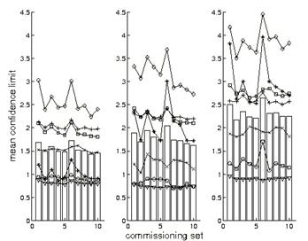
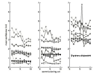
Next, we supplement the picture presented by the ranking approach with an examination of mean NXEGS performance. Fig. 3 gives the mean confidence limits, resolved according to type only; that is, the means we report there are over beam and depth (if relevant). In particular, for the depth independent error measures, j=1,2, we plot

(1)

as functions of i and l, while for the depth dependent error measures, j=3,…,7, we plot

(2)

as functions of the same indices.

One notes immediately in Fig. 3 that simulations tend to be most successful at SSD = 100 cm but are less so with increasing SSD. It is also readily seen that sets 1, 3, and 6 tend to give elevated results, consistent with what we have seen previously in the ranking approach, and that results for extended sets (1 through 5) differ little from results for brief sets (6 through 10), likewise consistent with our previous observations.

We roughly compare the relative overall success of the various commissionings by calculating the means of the means:

(3)

shown as bars in Fig. 3 and values in Table III. What are most important here are the relatively small differences in results between the stronger and weaker performers and the decreasing performance with increasing SSD. Table III presents two other slightly different views of the data. The first of these is an average of mean confidence limits normalized by data produced by set 9 (i=9) at SSD=100 cm (l=1) as follows:

(4)

This normalization has the effect of equally weighting in the average relative performances on each of the seven error measures, with the best performer according to this indicator, set 9, given unit score. The third view of mean performance shown in Table III uses the following average:

(5)

where min_il(x_ijl) selects the minimum of the set { x_ijl } for fixed j, so that for each i and l, mean confidence limits are normalized by the least corresponding confidence limit among the 30 available (irrespective of SSD).

Comparison of the orderings of the commissioning set types according to these various means in Table III shows minor differences, though each type of average we have used serves to distinguish the same set of better performers from the same set of poor performers. Given all this, the coherent picture emerges that it is sufficient to commission NXEGS with data taken at two rather than three SSDs and that, moreover, the beam models NXEGS generates tend to become more reliable with increasing size of the commissioning set, (discounting the use of three rather than two SSDs), though only slightly so and perhaps only up to a point. In addition, commissioning with minimally allowed set (sets 1 and 6), leads to elevated error across much of the range of our investigation, and so should probably be avoided. The concurrence of several different indicators on these points makes these conclusions especially strong.

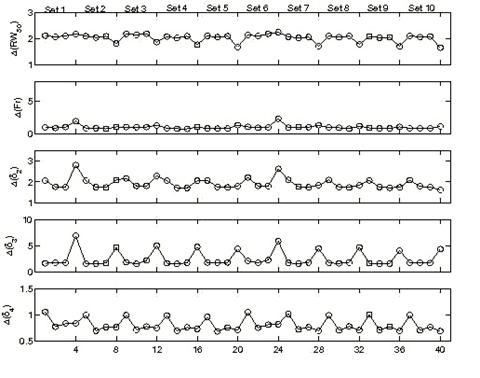
We gain a fuller understanding of the simulation results by examining their depth dependence, which we have so far suppressed. Fig. 4 shows mean values of the depth dependent confidence limits as a function of depth index and commissioning set for SSD = 100 cm. (Graphs for SSD = 110 and 120 cm are similar, but show elevation of the confidence limits with increasing SSD.) The means in this case are only over beams. Especially noteworthy are two features. The first is the presence in some of the graphs of elevated values occurring at d₄ = R₅₀ and sometimes at d₁ = 0.50 cm. Evidently, the confidence limits increase significantly at or near depths of R₅₀ (though, curiously, Δ(RW₅₀) decreases here), and this may suggest a trend of degraded performance with increasing depth. The other noteworthy feature concerns the two sets we have identified as stragglers, i.e. the minimal sets 1 and 6. Inspection shows that much of the increase in confidence limits associated with these sets is due to elevated values at d₄, and that performance at lesser depths is comparable to performance of the remaining sets.

Finally, it is important to note that any one simulation with NXEGS is in fact the result of two consecutive stochastic processes, namely the generation of the beam model from the commissioning set and the simulation of the beam with the model. It is of interest, therefore, to compare the results of two independent commissionings of NXEGS for the same beam, to see whether significant differences in beam simulation results arise. We arbitrarily choose the 6 MeV, 10×10 cm² beam, and commission NXEGS twice, using different random number generator seeds, with data sets 1 through 10, as described in Table I. This results in 10 pairs of corresponding beam models. With each model, we perform five independent simulations of dose in a water phantom, and extract PDDs and profiles as described earlier. Then for each of the two sets of commissionings we calculate Δ_ijkl =| μ_ijkl |+1.5 × σ_ijkl and compute ‹Δ_ijkl › as given in Eqns. (1,2) (here the beam index m is suppressed). Fig. 5 superposes ‹Δ_ijl › for both commissioning trials. For the most part, these results track each other satisfactorily. We have found that the typical absolute percentage difference between ‹Δ_il ›₁ and ‹Δ_il ›₂ (defined by Eqn. (3); subscripts designate the commissioning trials) is on the order of 1-10%, which suggests reasonable insensitivity of NXEGS to random differences in beam models.

We further substantiate this by examining the linear correlation between the set of values μ_ijkl (note that we do not take the absolute means here) for the first 10 commissionings and the corresponding values μ_ijkl from the second 10, and do the same for the two sets of values of both σ_ijkl and Δ_ijkl. In particular, for each fixed j, we form two ordered sets { μ_ijkl }₁ and { μ_ijkl }₂, one for each of the two sets of 10 commissionings, sharing the same ordering. If we regard one set as an independent variable and the second as the dependent variable, say, then we may examine the linear correlation between the two. In the absence of any differences between the beam models, this correlation should be perfect (because the five trial dose simulations per beam model were seeded identically in both cases), with r²=1, slope m=1, and intercept b=0, and differences should appear as deviations from this linearity. Again, in the absence of any differences between the beam models, the linear correlation between {σ_ijkl}₁ and {σ_ijkl}₂ and between {Δ_ijkl}₁ and {Δ_ijkl}₂ should likewise be perfect. The upper half of Table IV shows the results of performing the linear regressions as described for j=1,…,7. Nearly all the means are strongly correlated, while the standard deviations and confidence limits are moderately to strongly correlated, indicating that random differences in beam models are unlikely to perturb significantly our estimates of the reliability of NXEGS for electron beam calculation. Furthermore, one may get a qualitative sense of the relative contributions of statistical error due to simulation and statistical error due to commissioning by contrasting the above results with linear regressions on the sets { μ_ijkl}_1,a , {μ_ijkl}_1,b; {σ_ijkl}_1,a , {σ_ijkl}_1,b; and {Δ_ijkl}_1,a , {Δ_ijkl}_1,b , where the subscript '1' indicates that these data are generated from a single set of 10 beam models, while the subscripts 'a' and 'b' indicate two independent sets of five trials.

The lower half of Table IV displays these results for j=1,…,7. Deviations from linearity in the correlation between these sets are due to only random differences in simulation, while deviations in the previous case (upper half of Table IV) are due to random differences in both beam modeling and simulation. Thus, in a crude sense, the differences that one sees in Table IV are due to random errors in beam modeling alone. Fig. 6, which superposes for all j the sets {μ_ijkl}₁ versus {μ_ijkl}₂ and {Δ_ijkl}₁ versus {Δ_ijkl}₂, renders these results graphically.

4. Discussion

We have commissioned NXEGS software for electron beam dose calculation over a range of beam energies and applicator sizes using the program's automated commissioning feature. As a first test of the package, we have investigated how well NXEGS simulates the dose distributions from which the commissioning data were drawn. In summary, we have used confidence limits defined on seven measures of error to assess the performance of the program, finding that, regardless of the composition of commissioning sets, mean values of the seven confidence limits are typically less than 3 %/mm over most of the range of depths and SSDs we examined, though quality of the simulation is degraded with increasing SSD and at depths of about R₅₀. We have also found that commissioning requires dosimetric data collected at only two SSDs, that all the mean measures of confidence limits we used improve on the order of 20% when NXEGS is commissioned with sets significantly richer than the allowed minimal sets, and that, on average, commissioning with minimal sets tends to introduce excess error at greater, rather than lesser, depths. In addition, we note that, qualitatively, commissioning, itself a kind of Monte Carlo procedure, is robust against random variations, and so we have confidence in the generality of our other conclusions. Our continuing work will investigate the accuracy with which NXEGS can reproduce measured output factors, electron cutout factors, and dose distributions in complex geometries. Once the code is fully evaluated, our first clinical goal is to use it to compute electron cutout factors as an adjunct to routine measurement in phantoms as part of the treatment planning process, and ultimately as a replacement of such measurement.

At this point, it is useful to observe that as we have explored the behavior of a new dose calculation tool, we have contended with the problem of evaluating its relative overall performance across a number of its commissionings. A related but more typical problem is the evaluation of absolute overall performance of a treatment planning system as part of its commissioning or quality assurance. We propose, and plan to explore in subsequent work, that a modified version of some of the techniques we have used here may prove useful in such evaluations of absolute overall performance. For example, while the weightings and normalizations we have used here are simple and convenient, they are, we admit, open to the criticism of being naïvely chosen. A more measured approach to their choice, one into which are built carefully considered clinical requirements for the accuracy and precision of dose calculation, may result in an automated or semi-automated tool for the evaluation of treatment planning system performance that could supplement the clinicians' judgment.

Acknowledgements

This work was supported in part by NX Medical Software, LCC.

Competing interest

See Acknowledgement.

References

1. Rogers DWO, Faddegon BA, Ding GX, Ma C-M, Wei J, Mackie TR. Beam: a Monte Carlo code to simulate radiotherapy treatment units. Med Phys. 1995 ;22 :503 -24

2. Ma C-M, Faddegon BA, Rogers DWO, Mackie TR. Accurate characterization of Monte Carlo calculated electron beams for radiotherapy. Med Phys. 1996 ;24 :401 -416

3. Ma C-M, Jiang SB. Monte Carlo modeling of electron beams from medical accelerators. Phys Med Biol. 1999 ;44 :R157 -R189

4. Jiang SB, Kapur A, Ma C-M. Electron beam modeling and commissioning for Monte Carlo treatment planning. Med Phys. 2000 ;27 :180 -91

5. Almond PR, Biggs PJ, Coursey BM, Hanson WF, Saiful Huq M, Nath R, Rogers DWO. AAPM's TG-51 protocol for clinical reference dosimetry of high-energy photon and electron beams. Med Phys. 1999 ;26 :1847 -70

6. Venselaar J, Welleweerd H, Mijnheer B. Tolerances for the accuracy of photon beam dose calculations of treatment planning systems. Radiother Oncol. 2001 ;60 :191 -201

7. Van Dyk J, Barnett R B, Cygler JE, Schragge PC. Commissioning and quality assurance of treatment planning computers. Int J Radiation Oncology Biol Phys. 1993 ;26 :261 -273

8. Welleweerd J, van der Zee W. Dose calculation for asymmetric fields using Plato version 2_01. Radiother Oncol. 1998 ;48 (Suppl. 1) :134 -

9. Venselaar J, Welleweerd H. Application of a test package in an intercomparison of the performance of treatment planning systems used in a clinical setting. Radiother Oncol. 2001 ;60 :203 -213

Tables

Table I. Composition of 10 commissioning sets for each beam. P signifies central axis percent depth dose scan, D, X, and Y signify diagonal and primary axis scans. Labels d_k indicate depths, as in the text. Sets 1 through 5 consist data taken at SSD = 100, 110, and 120 cm. Sets 6 through 10 are identical to sets 1 through 5, respectively, but consist of data taken at SSD = 100 and 110 cm only.

Table II. Statistical summary of the ranking approach to determining optimal commissioning sets, sorted according to mean rank.

Table III. Values of mean mean confidence limits, given by Eqn. (3) and normalized means, given by Eqns. (4) and (5). Note that different normalization procedures lead to slightly different orderings

Table IV. The top half of the table reports on linear correlations between { μ_ijkl}₁ and {μ_ijkl}₂; {σ_ijkl}₁ and {σ_ijkl}₂; and {Δ_ijkl}₁ and {Δ_ijkl}₂, for two independent commissionings of the same beam with the same data. Deviations from linearity are due to random differences in beam modeling and simulation. The lower half reports on linear correlations between { μ_ijkl}_1,a and {μ_ijkl}_1,b; {σ_ijkl}_1,a and {σ_ijkl}_1,b; and {Δ_ijkl}_1,a and {Δ_ijkl}_1,b, defined in the text. Deviations from linearity are due to only random differences in simulation.

Fig. 1. A graphical summary of the seven indices of accuracy used to assess the quality of the simulations, after Venselaar, et al [6]. The left figure represents a typical PDD. The right figure represents a typical profile. Depth or in/crossplane displacement is the abscissa; the ordinate is relative dose.

Fig. 2 Rank distributions for each commissioning set. SSD = 100 cm. Histograms for SSD = 110, 120 cm are similar.

Fig. 3. Mean confidence limit for seven indicators. Circle, δ_1,pdd; × , δ _2,pdd; +, RW₅₀; *, Fr; square, δ ₂; diamond, δ ₃; triangle, δ ₄. The bars are the uniformly weighted means of the means. SSD = 100 cm (left), 110 cm, 120 cm (right). The units of the ordinate are % or mm, as appropriate.

Fig. 4. Mean confidence limit as a function of commissioning set and depth. The abscissa is 4(i-1)+k, where i is the commissioning set index and k is the depth index (1 through 4). Thus, points 1 through 4 correspond to set 1, depths d₁ through d₄, while points 37 through 40 correspond to set 10, depths d₁ through d₄, for example. SSD = 100 cm (top), 110 cm (middle), 120 cm (bottom).

Fig. 5. Comparison of mean confidence limit as in Fig. 3, but for two independent commissionings of the 6 MeV 10×10 cm² beam. Circle, δ_1,pdd; × , δ _2,pdd; +, RW₅₀; *, Fr; square, δ ₂; diamond, δ ₃; triangle, δ ₄. SSD = 100 cm (left), 110 cm, 120 cm (right). The units of the ordinate are % or mm, as appropriate. Dotted and solid lines differentiate the cases 1 and 2.

Fig 6. Left panels: correlation between { μ_ijkl}₁ and {μ_ijkl}₂ (top) and {Δ_ijkl}₁ and {Δ_ijkl}₂ (bottom) across independent commissionings. Right panels: correlation between { μ_ijkl}_1,a and {μ_ijkl}_1,b (top) and {Δ_ijkl}_1,a and {Δ_ijkl}_1,b (bottom) using the same commissionings but independent simulation, as described in the text.

Author biography

Joseph Both (Ph.D.) is a postdoctoral fellow in the physics division of the Department of Radiation Oncology at Stanford University School of Medicine. His research interests include radiation oncology physics, having pursued an earlier interest in the statistical mechanics of pattern formation. His current work is in patient specific Monte Carlo dose calculation and Monte Carlo modeling of robotic stereotactic radiosurgery devices.

Todd Pawlicki (Ph.D., DABR) is an assistant professor of radiation oncology physics at Stanford University School of Medicine. His research interests are primarily in Monte Carlo methods in radiotherapy, especially as related to patient specific dose calculation, treatment uncertainty, and electron and photon intensity modulated therapy. He has clinical interests in radiotherapy of the lung and head and neck, as well as stereotactic radiosurgery.

Corresponding address:

Joseph A. Both, Division of Radiation Physics, Department of Radiation Oncology, 875 Blake Wilbur Drive, Stanford, CA, 94305-5847, USA.

Email: jbothstanford.edu. Tel: 650 498 4074.

Received 2004-3-02
Accepted 2004-5-12
Published 2004-6-01

Citation styles

©2024 Ivyspring International Publisher. Terms of use